When a radar sends out radio waves, airplanes are not the only things that send echoes back. Land, sea, raindrops and birds return the waves too. Among all those echoes, how does the radar find one small target?
The key is motion. The ground stays put, and the target moves. This article looks at two ways to keep only the moving echoes by using a small change in waves reflected from moving objects: the Doppler shift. It then follows how U.S. weather radar adopted the idea, and ends with Doppler lidar, which uses the same principle with light.
The basics of how radar finds distance from the round-trip time of a radio wave are in "Radar: measuring distance and motion with radio waves."
A small target hidden among echoes
The echoes a radar does not want are called clutter. Land, sea, rain and birds are typical sources. Clutter comes back from the same range and angle cell as the target. So range and direction alone cannot pull the two apart.
Clutter is often much stronger, too. Radar course notes from MIT Lincoln Laboratory state that the radar cross section (RCS) of clutter can exceed that of the targets of interest by more than 50 dB. Its character also changes with the terrain, land or sea, and with the weather.
Still, there is one opening. Seen from a radar on the ground, targets move and clutter does not. A radar on an aircraft is a different case. The radar itself is moving, so its own motion has to be taken into account.
Higher when closing, lower when opening
When an ambulance passes with its siren on, the pitch drops. The frequency you hear changes when the source or the listener moves. This is the Doppler effect, and the actual change in frequency is the Doppler shift. The name comes from the Austrian physicist Christian Johann Doppler (1803–1853).
Moving closer gives a higher frequency, and moving apart gives a lower one. The effect is not limited to sound. It happens with any wave, light and radio waves included, whenever the observer and the source move relative to each other. Police radar that measures the speed of cars works on this principle.
With radar, the target is the one sending the wave back. An echo from a closing target has its crests packed closer, so its frequency rises. An echo from an opening target has its crests spread apart, so its frequency falls. An echo from the still ground is the same as what was sent.
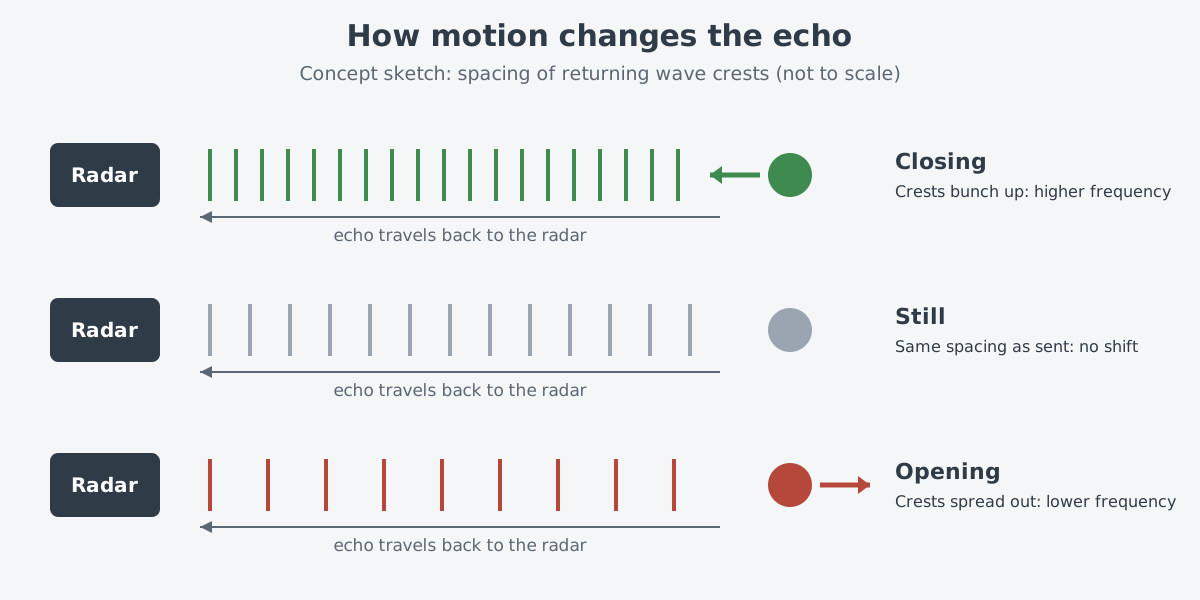
The sketch exaggerates the change. The real change is tiny. Take an example from the Lincoln Laboratory notes. For a 2800 MHz radar, the Doppler frequency grows by about 1 kHz for every 40 m/s of a target's speed toward it.
That is roughly one part in a few million of the transmitted frequency. The U.S. weather radar WSR-88D picks up this motion as a change in the phase of the returning pulse.
Only the speed along the line of sight
The Doppler shift tells you whether a target is moving toward the radar or away from it, and how fast it is moving in that direction. This speed, measured along the line between radar and target, is called radial velocity. Whatever direction an aircraft is actually flying, the part a radar gets directly from the Doppler shift is this one component.
The velocity display of a weather radar shows this well. According to the National Weather Service (NWS), the radar's computers calculate the Doppler shift in each echo. From it they judge whether the rain is coming closer or heading off, and at what speed, and then color it to match. Red usually means moving away from the radar, and green means moving toward it.
Erasing still echoes: moving target indication
There are two main ways to remove clutter with the Doppler shift: moving target indication (MTI) and pulse Doppler (PD). Both lean on the Doppler shift to filter out clutter and make moving targets easier to find. The smaller the target, the more clutter suppression it needs.
MTI is the simpler of the two. It uses only two or three pulses and does one job: separating moving targets from clutter. It does not tell you how fast a target is moving.
The simplest form subtracts two pulses. Take the echo of one pulse and subtract the echo of the pulse before it. Echoes from still ground and buildings are the same both times, so they cancel. A moving target's echo changes in amplitude from pulse to pulse because of its Doppler shift.
So something is left after the subtraction, and the radar treats that residue as a target.
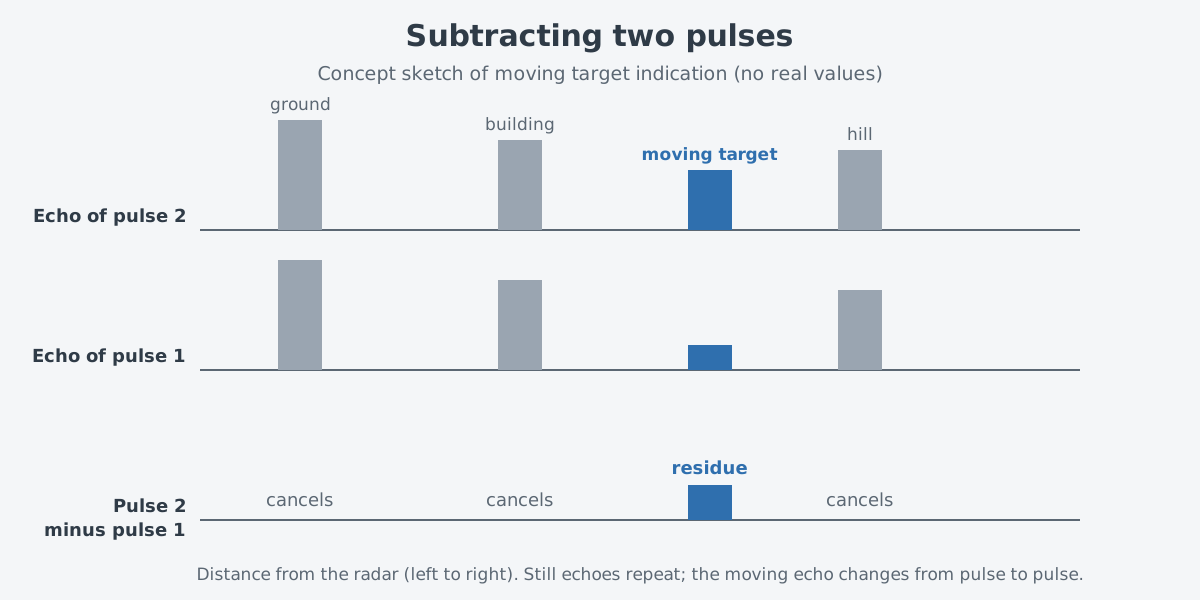
It is a bit like taking two photos of the same spot a moment apart and subtracting one from the other, so that only what moved remains. The real process is different. A radar does not compare shapes; it compares echoes from the same range cell, and the reason a target's echo changes between pulses is the Doppler shift.
There are limits, too. MTI has only a limited ability to suppress rain clutter.
Sorting by speed: pulse Doppler
Pulse Doppler goes a step further. It collects many pulses, passes them through a bank of Doppler filters, and sorts the echoes into speed bins. Besides removing clutter, it can estimate a target's radial velocity in fine detail.
The moving target detector (MTD) in the Lincoln Laboratory notes is one example. It uses a Doppler filter bank and two pulse repetition frequencies to find aircraft in ground clutter or rain. Birds and ground traffic are filtered out in later processing with Doppler velocity and a clutter map.
Sending pulses over and over has a cost. The number of pulses sent per second is the pulse repetition frequency (PRF). Two targets whose Doppler frequencies differ by a whole multiple of the PRF cannot be told apart.
Range has the same kind of problem. if the next pulse goes out before all echoes of the last one are back, range becomes confused. These problems are called ambiguities.
Following the formulas in the course notes, a higher PRF widens the range of speeds you can measure without confusion but narrows the range of distances. It is hard to widen both at once. So radars send several bursts of pulses with different PRFs to resolve both ambiguities. Radars on aircraft also use waveforms with several PRFs to suppress clutter.
How weather radar got there
The rain velocity maps in weather forecasts also come from Doppler radar. The history page of the National Severe Storms Laboratory (NSSL) traces the path.
In 1956, Cornell Aeronautical Laboratory built a 3 cm continuous-wave Doppler radar. It used one antenna to transmit and another to receive. It was built to catch the very high winds in tornadoes, but it could not tell how far away the tornado was.
In 1964, NSSL engineers changed this radar to send pulses. Because it could receive echoes between pulses, it no longer needed two antennas, and the distance problem was solved. In 1971, the NSSL experimental Doppler radar began operating.
On May 24, 1973, an NSSL team filmed the whole life of a tornado in a storm that the Doppler radar was scanning. Comparing the film with the radar data, researchers found a pattern showing that the tornado was forming before it appeared on film. They named it the Tornado Vortex Signature (TVS), and NSSL writes that this discovery eventually led to a nationwide network of Doppler radars.
In 1976, the Joint Doppler Operational Project (JDOP) set out to show that Doppler radar could improve warnings for severe thunderstorms and tornadoes. This led to a decision in 1979. The NWS, the U.S. Air Force's Air Weather Service and the Federal Aviation Administration (FAA) agreed to build Doppler capability into their future operational radars.
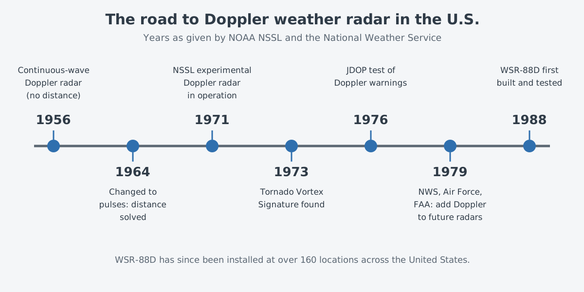
The radar that came out of this is the WSR-88D. According to the NWS, it was first built and tested in 1988 and has since gone into service at more than 160 U.S. sites, Alaska and Hawaii among them. Motion along the beam gives wind speed, and the NWS says this ability to "see" the wind lets it spot tornadoes forming and warn people earlier.
Where this meets lasers: Doppler lidar
The Doppler effect also happens with light. So some devices send laser light instead of radio waves and read the Doppler shift of the light that comes back. They are called Doppler lidars.
A NOAA instrument called the High Resolution Doppler Lidar (HRDL) measured and mapped air velocities; it has since been retired. NOAA is the U.S. National Oceanic and Atmospheric Administration. What it produced were range-resolved line-of-sight velocities. In other words, it measured the same kind of speed a Doppler radar does, but with light.
The idea has also gone to space. The European Space Agency (ESA) flew Aeolus with a Doppler wind lidar as its only large instrument. It became the first satellite mission that gathered wind profiles for the whole Earth. It was launched on August 22, 2018, and the mission ended on July 28, 2023.
The basics of measuring distance with lasers continue in "Measuring with lasers: range finding and lidar basics."
What to read next
- Radar: measuring distance and motion with radio waves: how round-trip time gives distance, and the basics of the Doppler effect.
- Drone or bird: what sensors look at: the small patterns on top of a body's Doppler shift, called micro-Doppler.
- Measuring with lasers: range finding and lidar basics: what changes when the same idea moves to light.
- Synthetic aperture radar: images from radio waves: a radar that uses the Doppler shift to sharpen its images.