Radio towers and TV transmitters send out signals day and night. Those waves do not stop at the receivers in people's homes. They also hit aircraft passing overhead, and part of that energy scatters in every direction.
Some radars see the sky by picking out only those scattered echoes. A passive radar has no transmitter of its own and borrows signals that someone else sends. This article looks at how it can measure range without a transmitter, what its hardest problem is, and how the idea goes back to the early days of radar.
A radar without a transmitter
An ordinary radar sends out radio waves and listens for what bounces back. A passive radar skips the sending. It treats broadcast and communication signals that are already in the air as an illuminator of opportunity (IoO), and it receives the part of those signals reflected by a target.
Because it emits no radar signal, the receiving site does not give away its position by radio. That is the main reason passive radar has drawn interest from both researchers and the military.
Another name for the same idea is passive coherent location (PCL). It usually means a system in which a third party does the transmitting and the designer builds only the receiver. It is sometimes called a "hitchhiking" mode, since the radar rides on someone else's transmitter.
One point is easy to mix up. Equipment that listens to signals a target sends out by itself is listening for something different. A passive radar listens for someone else's signal after it has bounced off the target.
Separate transmitter and receiver: an ellipse instead of a circle
The Institute of Electrical and Electronics Engineers (IEEE) defines a bistatic radar as one that transmits and receives with antennas at different locations. The distance between the two sites is called the baseline. No rule says how far apart they must be, and with a very short baseline the system behaves almost like a monostatic radar, which sends and receives from one place. Since the broadcast station and the receiving site are apart, a passive radar is bistatic by nature.
A monostatic radar measures range from the round-trip time. If you join all the points whose echoes return at the same time, you get a circle centered on the radar. Once the two sites are apart, the picture changes. What matters now is the path from the transmitter to the target (R₁) plus the path from the target to the receiver (R₂).
The bistatic range that a passive radar measures is the sum of those two paths minus the baseline. The baseline can be known in advance once the station's position is known.
R = R₁ + R₂ − L
R is the bistatic range, R₁ is the distance from transmitter to target, R₂ is the distance from target to receiver, and L is the baseline.
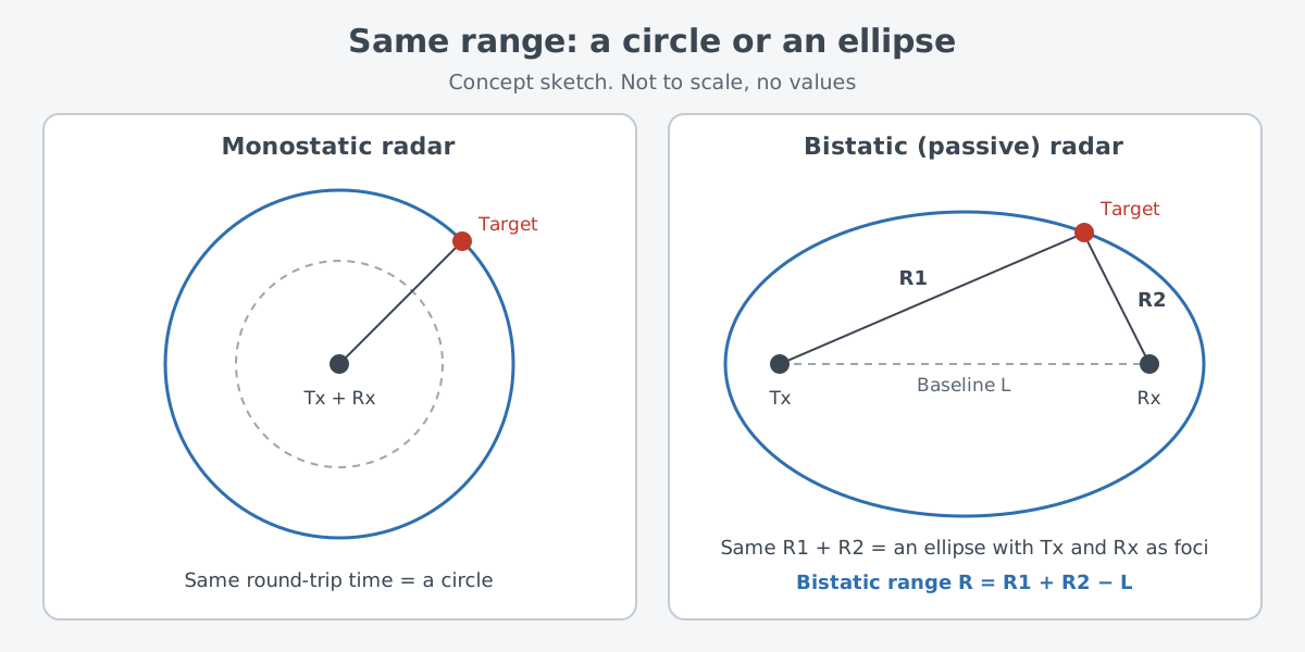
Points with the same total path lie on an ellipse whose two foci are the transmitter and the receiver. It is the same shape you draw by tying a loop of string to two pins and pulling it tight with a pencil. Real space has three dimensions, so the ellipse becomes an ellipsoid, shaped a bit like a rugby ball.
One range value only says the target is somewhere on that ellipsoid. To fix its position, the radar also measures the direction the echo comes from and finds where that direction meets the ellipsoid. Another option is to use several transmitter–receiver pairs and find the point where their ellipsoids cross.
Listening with two ears: reference signal and echo
Borrowing a broadcast creates a problem. The receiving side does not know in advance exactly what the station has just sent. So a passive radar records the original signal and the echo separately and compares the two.
The receiver has two channels. The reference channel picks up the signal arriving straight from the station, and the surveillance channel picks up what comes from the patch of sky being watched. The radar delays the reference signal step by step and shifts its frequency by a Doppler shift, then checks how well each version matches the surveillance signal. This calculation is called the cross ambiguity function (CAF), and targets show up at the delay and frequency shift where the match is strong.
The reference channel also keeps the transmitter and receiver in step. A radar at one site can time both sending and receiving from a single oscillator, but once the two are apart this becomes much harder. Bistatic radars may use synchronized atomic clocks or a signal such as GPS, while PCL systems usually rely on the reference signal received straight from the transmitter.
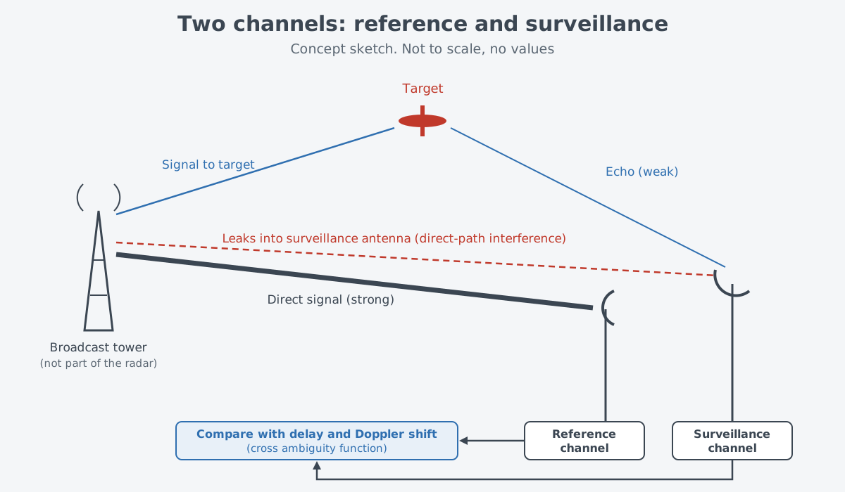
The biggest headache is that the station's signal also leaks straight into the surveillance channel. This is called direct-path interference (DPI). It can be far stronger than the target echoes, and unless steps are taken it drowns them out.
It is a bit like trying to hear a faint, distant echo while a loudspeaker blares right next to you. The difference is that the echo is a slightly delayed repeat of the loudspeaker's own sound. Comparing it with the original signal from the reference channel gives the radar a way to pick it out.
Which signals get borrowed
Published research lists a wide range of illuminators of opportunity. They include FM radio, digital audio broadcasting (DAB), digital terrestrial TV (DVB-T), mobile networks such as GSM and LTE, satellite navigation (GNSS), satellite TV (DVB-S), wireless LAN, and 5G.
None of these signals were made for radar. Their waveforms are designed for broadcasting or communication, and the receiving side cannot change any of the transmission settings. Finding a weak target echo in them therefore takes complex signal processing.
The choice of signal also changes what the radar can see. Range resolution is the smallest difference in range at which two targets can still be told apart. For a given bistatic angle, it is set by the bandwidth of the borrowed signal.
A 2023 review paper in Sensors gives typical values at a bistatic angle of 60°. They are 1.0–3.5 km for FM radio, 800 m for GSM, 100 m for DAB, 22 m for DVB-T, 9 m for LTE, and 7 m for GNSS.
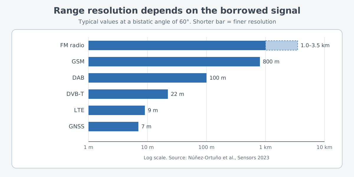
How far the radar can see depends on the transmit power. Among them, FM and DVB-T transmit with the most power, and GNSS and DVB-S with the least. So the signal with the finest resolution is not necessarily the one that reaches farthest. In practice the choice weighs the kind of target and how it moves, the resolution wanted, the area to be covered, and whether a usable station exists nearby.
Strengths and difficulties
Start with the strengths: a passive radar sends nothing, so placing a receiver needs no frequency allocation. That makes it usable even in crowded areas where radio interference is a problem. It is also smaller and cheaper than an active radar doing a similar job. Hugh Griffiths of University College London (UCL), in an IEEE society lecture abstract, adds that the receiving equipment can be simple and low in cost.
The difficulties are just as clear. Where the transmitter stands and what it sends are out of the radar designer's hands. The geometry is more complex than for a single-site radar, and the transmitter and receiver must be synchronized in some way. How clutter, the unwanted reflections from land or sea, behaves in a bistatic setup is also still poorly understood.
Maturity is another question. In a 2005 paper, Baker and Griffiths wrote that PCL should be seen as an emerging technology rather than a mature one. Many bistatic and multistatic systems have been built and tested, but very few have gone past the "technology demonstrator" stage.
Interest in the field has also come and gone. Nicholas Willis noted in his book Bistatic Radar that attention to bistatic radar rises and falls on a cycle of about fifteen years.
From Daventry in 1935 to the Second World War
Researchers have worked on and built bistatic and multistatic radars ever since radar's earliest days. According to the timeline of the Royal Air Force Museum (RAF Museum), the first practical demonstration of detecting aircraft by radio took place on 26 February 1935. The test followed proposals by R.A. Watson Watt, head of the Radio Department at the National Physical Laboratory.
The test itself looks a lot like the subject of this article. Signals from a 10 kW transmitter at Daventry bounced off a Royal Air Force Handley Page Heyford bomber. Staff of the Radio Research Station at Slough picked up the aircraft with experimental equipment set up at Weedon in Northamptonshire. The transmitter and the receiving equipment stood in different places, so by the definition above this was a bistatic arrangement, with a maximum detection range estimated at about 8 miles.
During the Second World War, Germany borrowed another side's radar: it used Britain's Chain Home radars as the illuminator for a bistatic system called Klein Heidelberg. Griffiths and Willis analyzed the system in a 2010 IEEE journal paper. They found its performance impressive, with Allied bombers detected at more than 300 km. Even so, it came into operation too late in the war to do much for German air defense.
Later, as broadcast and communication signals multiplied, there were more signals to borrow. The 2005 paper gives examples of reported operational systems, including Lockheed Martin's "Silent Sentry" for air and space surveillance and the Manastash Ridge radar used for upper-atmosphere and ionosphere research. Scientific uses such as oceanography and mapping lightning paths inside thunderstorms are listed as well.
What to read next
- Radar: measuring distance and motion with radio waves: how an ordinary radar, with transmitter and receiver in one place, measures range and speed from round-trip time and the Doppler effect.
- Doppler Radar: Picking Out Things That Move: a closer look at the frequency shift a passive radar tries out when it matches the reference signal.
- Measuring with lasers: range finding and lidar basics: measuring distance from the return time of light instead of radio waves.